Section 3.4 Derivatives as Rates of Change
Learning Objectives.
Determine a new value of a quantity from the old value and the amount of change.
Calculate the average rate of change and explain how it differs from the instantaneous rate of change.
Apply rates of change to displacement, velocity, and acceleration of an object moving along a straight line.
Predict the future population from the present value and the population growth rate.
Use derivatives to calculate marginal cost and revenue in a business situation.
In this section we look at some applications of the derivative by focusing on the interpretation of the derivative as the rate of change of a function. These applications include acceleration and velocity in physics, population growth rates in biology, and marginal functions in economics.
Subsection 3.4.1 Amount of Change Formula
One application for derivatives is to estimate an unknown value of a function at a point by using a known value of a function at some given point together with its rate of change at the given point. If \(f(x)\) is a function defined on an interval \([a,a+h],\) then the amount of change of \(f(x)\) over the interval is the change in the \(y\) values of the function over that interval and is given by
The average rate of change of the function \(f\) over that same interval is the ratio of the amount of change over that interval to the corresponding change in the \(x\) values. It is given by
As we already know, the instantaneous rate of change of \(f(x)\) at \(a\) is its derivative
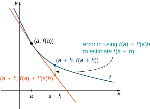
For small enough values of \(h,f'(a)\approx \frac{f(a+h)-f(a)}{h}.\) We can then solve for \(f(a+h)\) to get the amount of change formula:
We can use this formula if we know only \(f(a)\) and \(f'(a)\) and wish to estimate the value of \(f(a+h).\) For example, we may use the current population of a city and the rate at which it is growing to estimate its population in the near future. As we can see in Figure 3.91, we are approximating \(f(a+h)\) by the \(y\) coordinate at \(a+h\) on the line tangent to \(f(x)\) at \(x=a.\) Observe that the accuracy of this estimate depends on the value of \(h\) as well as the value of \(f'(a).\)

Note 3.92.
Here is an interesting demonstration 1 of rate of change.
Example 3.93. Estimating the Value of a Function.
If \(f(3)=2\) and \(f'(3)=5,\) estimate \(f(3.2).\)
Begin by finding \(h.\) We have \(h=3.2-3=0.2.\) Thus,
Checkpoint 3.94.
Given \(f(10)=-5\) and \(f'(10)=6,\) estimate \(f(10.1).\)
Subsection 3.4.2 Motion along a Line
Another use for the derivative is to analyze motion along a line. We have described velocity as the rate of change of position. If we take the derivative of the velocity, we can find the acceleration, or the rate of change of velocity. It is also important to introduce the idea of speed, which is the magnitude of velocity. Thus, we can state the following mathematical definitions.
Definition 3.95.
Let \(s(t)\) be a function giving the position of an object at time \(t.\)
The velocity of the object at time \(t\) is given by \(v(t)=s'(t).\)
The speed of the object at time \(t\) is given by \(|v(t)|.\)
The acceleration of the object at \(t\) is given by \(a(t)=v'(t)=s''(t).\)
Example 3.96. Comparing Instantaneous Velocity and Average Velocity.
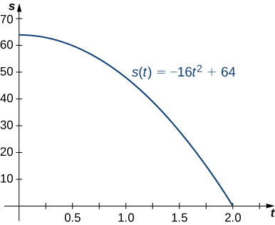
A ball is dropped from a height of 64 feet. Its height above ground (in feet) \(t\) seconds later is given by \(s(t)=-16t^2+64.\)

What is the instantaneous velocity of the ball when it hits the ground?
What is the average velocity during its fall?
The first thing to do is determine how long it takes the ball to reach the ground. To do this, set \(s(t)=0.\) Solving \(-16t^2+64=0,\) we get \(t=2,\) so it take 2 seconds for the ball to reach the ground.
The instantaneous velocity of the ball as it strikes the ground is \(v(2).\) Since \(v(t)=s'(t)=-32t,\) we obtain \(v(t)=-64 \text{ ft/s }.\)
The average velocity of the ball during its fall is
\begin{equation*} v_{\text{ ave }}=\frac{s(2)-s(0)}{2-0}=\frac{0-64}{2}=-32 \text{ ft/s }. \end{equation*}
Subsection 3.4.3 Population Change
In addition to analyzing velocity, speed, acceleration, and position, we can use derivatives to analyze various types of populations, including those as diverse as bacteria colonies and cities. We can use a current population, together with a growth rate, to estimate the size of a population in the future. The population growth rate is the rate of change of a population and consequently can be represented by the derivative of the size of the population.
Definition 3.97.
If \(P(t)\) is the number of entities present in a population, then the population growth rate of \(P(t)\) is defined to be \(P'(t).\)
Example 3.98. Estimating a Population.
The population of a city is tripling every 5 years. If its current population is 10,000, what will be its approximate population 2 years from now?
Let \(P(t)\) be the population (in thousands) \(t\) years from now. Thus, we know that \(P(0)=10\) and based on the information, we anticipate \(P(5)=30.\) Now estimate \(P'(0),\) the current growth rate, using
By applying (3.4.1) to \(P(t),\) we can estimate the population 2 years from now by writing
thus, in 2 years the population will be 18,000.
Checkpoint 3.99.
The current population of a mosquito colony is known to be 3,000; that is, \(P(0)=3,000.\) If \(P'(0)=100,\) estimate the size of the population in 3 days, where \(t\) is measured in days.
Subsection 3.4.4 Changes in Cost and Revenue
In addition to analyzing motion along a line and population growth, derivatives are useful in analyzing changes in cost, revenue, and profit. The concept of a marginal function is common in the fields of business and economics and implies the use of derivatives. The marginal cost is the derivative of the cost function. The marginal revenue is the derivative of the revenue function. The marginal profit is the derivative of the profit function, which is based on the cost function and the revenue function.
Definition 3.100.
If \(C(x)\) is the cost of producing \(x\) items, then the marginal cost \(MC(x)\) is \(MC(x)=C'(x).\)
If \(R(x)\) is the revenue obtained from selling \(x\) items, then the marginal revenue \(MR(x)\) is \(MR(x)=R'(x).\)
If \(P(x)=R(x)-C(x)\) is the profit obtained from selling \(x\) items, then the marginal profit \(MP(x)\) is defined to be \(MP(x)=P'(x)=MR(x)-MC(x)=R'(x)-C'(x).\)
We can roughly approximate
by choosing an appropriate value for \(h.\) Since \(x\) represents objects, a reasonable and small value for \(h\) is 1. Thus, by substituting \(h=1,\) we get the approximation \(MC(x)=C'(x)\approx C(x+1)-C(x).\) Consequently, \(C'(x)\) for a given value of \(x\) can be thought of as the change in cost associated with producing one additional item. In a similar way, \(MR(x)=R'(x)\) approximates the revenue obtained by selling one additional item, and \(MP(x)=P'(x)\) approximates the profit obtained by producing and selling one additional item.
Example 3.101. Applying Marginal Revenue.
Assume that the number of barbeque dinners that can be sold, \(x,\) can be related to the price charged, \(p,\) by the equation \(p(x)=9-0.03x,0\leq x\leq 300.\)
In this case, the revenue in dollars obtained by selling \(x\) barbeque dinners is given by
Use the marginal revenue function to estimate the revenue obtained from selling the 101st barbeque dinner. Compare this to the actual revenue obtained from the sale of this dinner.
First, find the marginal revenue function: \(MR(x)=R'(x)=-0.06x+9.\)
Next, use \(R'(100)\) to approximate \(R(101)-R(100),\) the revenue obtained from the sale of the 101st dinner. Since \(R'(100)=3,\) the revenue obtained from the sale of the 101st dinner is approximately \$3.
The actual revenue obtained from the sale of the 101st dinner is
The marginal revenue is a fairly good estimate in this case and has the advantage of being easy to compute.
Checkpoint 3.102.
Suppose that the profit obtained from the sale of \(x\) fish-fry dinners is given by \(P(x)=-0.03x^2+8x-50.\) Use the marginal profit function to estimate the profit from the sale of the 101st fish-fry dinner.
Subsection 3.4.5 Key Concepts
Using \(f(a+h)\approx f(a)+f'(a)h,\) it is possible to estimate \(f(a+h)\) given \(f'(a)\) and \(f(a).\)
The rate of change of position is velocity, and the rate of change of velocity is acceleration. Speed is the absolute value, or magnitude, of velocity.
The population growth rate and the present population can be used to predict the size of a future population.
Marginal cost, marginal revenue, and marginal profit functions can be used to predict, respectively, the cost of producing one more item, the revenue obtained by selling one more item, and the profit obtained by producing and selling one more item.
This book is a custom edition based on OpenStax Calculus Volume 1. You can download the original for free at https://openstax.org/details/books/calculus-volume-1.
http://www.openstax.org/l/20_chainrule