Linear Approximations

Section 4.2 Linear Approximations

Learning Objectives.

Describe the linear approximation to a function at a point.
Write the linearization of a given function.

We have just seen how derivatives allow us to compare related quantities that are changing over time. In this section, we examine another application of derivatives: the ability to approximate functions locally by linear functions. Linear functions are the easiest functions with which to work, so they provide a useful tool for approximating function values. In addition, the ideas presented in this section are generalized later in the text when we study how to approximate functions by higher-degree polynomials .

🔗

Subsection 4.2.1 Linear Approximation of a Function at a Point

🔗

Consider a function

f

that is differentiable at a point

x = a .

Recall that the tangent line to the graph of

f

a

is given by the equation

y = f (a) + f^{'} (a) (x - a) .

🔗

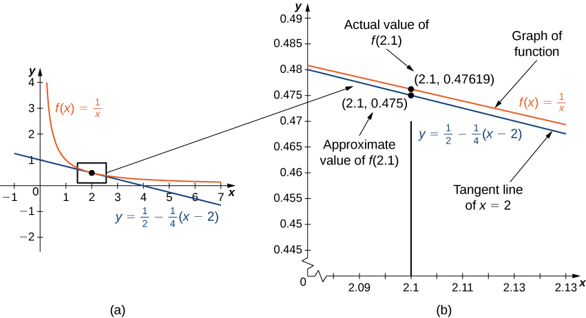
For example, consider the function

f (x) = \frac{1}{x}

a = 2.

Since

f

is differentiable at

x = 2

and

f^{'} (x) = - \frac{1}{x^{2}},

we see that

f^{'} (2) = - \frac{1}{4} .

Therefore, the tangent line to the graph of

f

a = 2

is given by the equation

y = \frac{1}{2} - \frac{1}{4} (x - 2) .

🔗

Figure 4.11(a) shows a graph of

f (x) = \frac{1}{x}

along with the tangent line to

f

x = 2.

Note that for

x

near 2, the graph of the tangent line is close to the graph of

f .

As a result, we can use the equation of the tangent line to approximate

f (x)

for

x

near 2. For example, if

x = 2.1,

the

y

value of the corresponding point on the tangent line is

y = \frac{1}{2} - \frac{1}{4} (2.1 - 2) = 0.475 .

🔗

The actual value of

f (2.1)

is given by

f (2.1) = \frac{1}{2.1} \approx 0.47619 .

🔗

Therefore, the tangent line gives us a fairly good approximation of

f (2.1)

(Figure 4.11(b)). However, note that for values of

x

far from 2, the equation of the tangent line does not give us a good approximation. For example, if

x = 10,

the

y

-value of the corresponding point on the tangent line is

y = \frac{1}{2} - \frac{1}{4} (10 - 2) = \frac{1}{2} - 2 = - 1.5,

🔗

whereas the value of the function at

x = 10

f (10) = 0.1 .

"This figure has two parts a and b. In figure a, the line f(x) = 1/x is shown with its tangent line at x = 2. In figure b, the area near the tangent point is blown up to show how good of an approximation the tangent is near x = 2." — 🔗
Figure 4.11. (a) The tangent line to $f (x) = 1 / x$ at $x = 2$ provides a good approximation to $f$ for $x$ near 2. (b) At $x = 2.1,$ the value of $y$ on the tangent line to $f (x) = 1 / x$ is 0.475. The actual value of $f (2.1)$ is $1 / 2.1,$ which is approximately 0.47619.

🔗

In general, for a differentiable function

f,

the equation of the tangent line to

f

x = a

can be used to approximate

f (x)

for

x

near

a .

Therefore, we can write

f (x) \approx f (a) + f^{'} (a) (x - a) for x near a .

🔗

We call the linear function

\begin{matrix} (4.2.1) & L (x) = f (a) + f^{'} (a) (x - a) \end{matrix}

🔗

the linear approximation, or tangent line approximation, of

f

x = a .

This function

L

is also known as the linearization of

f

x = a .

🔗

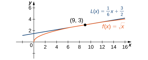
To show how useful the linear approximation can be, we look at how to find the linear approximation for

f (x) = \sqrt{x}

x = 9.

🔗

Example 4.12.

Find the linear approximation of $f (x) = \sqrt{x}$ at $x = 9$ and use the approximation to estimate $\sqrt{9.1} .$

Solution.

Since we are looking for the linear approximation at $x = 9,$ using (4.2.1) we know the linear approximation is given by

L (x) = f (9) + f^{'} (9) (x - 9) .

We need to find $f (9)$ and $f^{'} (9) .$

\begin{aligned} f (x) = \sqrt{x} & ⟹ & f (9) = \sqrt{9} = 3 \\ f^{'} (x) = \frac{1}{2 \sqrt{x}} & ⟹ & f^{'} (9) = \frac{1}{2 \sqrt{9}} = \frac{1}{6} \end{aligned}

Therefore, the linear approximation is given by Figure 4.13.

L (x) = 3 + \frac{1}{6} (x - 9)

Using the linear approximation, we can estimate $\sqrt{9.1}$ by writing

\sqrt{9.1} = f (9.1) \approx L (9.1) = 3 + \frac{1}{6} (9.1 - 9) \approx 3.0167 .

"The function f(x) = the square root of x is shown with its tangent at (9, 3). The tangent appears to be a very good approximation from x = 6 to x = 12." — Figure 4.13. The local linear approximation to $f (x) = \sqrt{x}$ at $x = 9$ provides an approximation to $f$ for $x$ near 9.

🔗

Checkpoint 4.15.

Find the local linear approximation to $f (x) = \sqrt[3]{x}$ at $x = 8.$ Use it to approximate $\sqrt[3]{8.1}$ to five decimal places.

Hint.

$L (x) = f (a) + f^{'} (a) (x - a)$

Solution.

$L (x) = 2 + \frac{1}{12} (x - 8);$ 2.00833

🔗

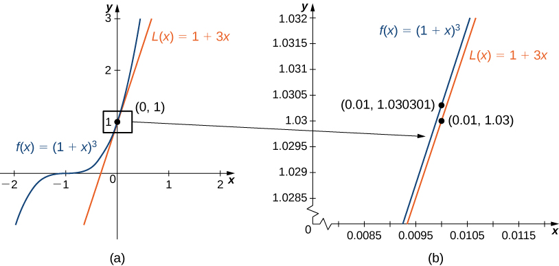
Linear approximations may be used in estimating roots and powers. In the next example, we find the linear approximation for

f (x) = (1 + x)^{n}

x = 0,

which can be used to estimate roots and powers for real numbers near 1. The same idea can be extended to a function of the form

f (x) = (m + x)^{n}

to estimate roots and powers near a different number

m .

🔗

Example 4.16. Approximating Roots and Powers.

Find the linear approximation of $f (x) = (1 + x)^{n}$ at $x = 0.$ Use this approximation to estimate $(1.01)^{3} .$

Solution.

The linear approximation at $x = 0$ is given by

L (x) = f (0) + f^{'} (0) (x - 0) .

Because

\begin{aligned} f (x) = (1 + x)^{n} & ⟹ & f (0) = 1 \\ f^{'} (x) = n (1 + x)^{n - 1} & ⟹ & f^{'} (0) = n, \end{aligned}

the linear approximation is given by Figure 4.17(a).

L (x) = 1 + n (x - 0) = 1 + n x

We can approximate $(1.01)^{3}$ by evaluating $L (0.01)$ when $n = 3.$ We conclude that

(1.01)^{3} = f (1.01) \approx L (1.01) = 1 + 3 (0.01) = 1.03 .

"This figure has two parts a and b. In figure a, the line f(x) = (1 + x)3 is shown with its tangent line at (0, 1). In figure b, the area near the tangent point is blown up to show how good of an approximation the tangent is near (0, 1)." — Figure 4.17. (a) The linear approximation of $f (x)$ at $x = 0$ is $L (x) .$ (b) The actual value of ${1.01}^{3}$ is 1.030301. The linear approximation of $f (x)$ at $x = 0$ estimates ${1.01}^{3}$ to be 1.03.

🔗

Checkpoint 4.18.

Find the linear approximation of $f (x) = (1 + x)^{4}$ at $x = 0$ without using the result from the preceding example.

Hint.

$f^{'} (x) = 4 (1 + x)^{3}$

Solution.

$L (x) = 1 + 4 x$

🔗

Example 4.19.

The profit equation for a certain product is given by $P (x) = \frac{20}{\sqrt{x + 2}}$ where $x$ is the number of units sold. Use the linear approximation formula of $P$ to estimate the changes in profit as $x$ changes from 98 to 101.

Solution.

Using the linear approximation at $x = 98,$

L (x) = P (98) + P^{'} (98) (x - 98)

Thus,

\begin{aligned} P (x) & = 20 (x + 2)^{- 1 / 2} \\ P^{'} (x) & = - 10 (x + 2)^{- 3 / 2} = \frac{- 10}{(x + 2)^{3 / 2}} . \end{aligned}

We see that

\begin{aligned} P (x) = \frac{20}{\sqrt{x + 2}} & ⟹ & P (98) = \frac{20}{\sqrt{100}} = 2 \\ P^{'} (x) = \frac{- 10}{(x + 2)^{3 / 2}} & ⟹ & P^{'} (98) = \frac{- 10}{(100)^{3 / 2}} = - 0.01 \end{aligned}

Therefore, the linear approximation of $P$ at $x = 98$ is given by

L (x) = 2 - 0.01 (x - 98)

The estimate for $P (101)$ is given by

P (101) \approx L (101) = 2 - 0.01 (101 - 98) = 1.97 .

Thus, our estimate for the changes in profit as $x$ changes from 98 to 101 is

P (101) - P (98) \approx 1.97 - 2 = - 0.03 .

That is, profit decreased by about 3 cents. Note that the true value for the changes in profit as $x$ changes from 98 to 101 is

P (101) - P (98) = 1.970658556 - 2 = - 0.0293414437 .

🔗

Checkpoint 4.20.

The demand equation for a box of tea is given by $p (x) = \frac{30}{\sqrt{x}}$ where $x$ is the number of boxes of tea sold. Use the linear approximation formula of $p$ to estimate the changes in demand as $x$ changes from 9 to 10.

Hint.

$L (x) = f (a) + f^{'} (a) (x - a)$

Solution.

L (x) = 10 - \frac{5}{9} (x - 9)

p (10) \approx L (10) = 9. \overset{―}{4} ⟹ p (10) - p (9) \approx 9. \overset{―}{4} - 10 = - 0. \overset{―}{5} \approx - $ 0.56 .

🔗

Subsection 4.2.2 Average Cost

🔗

Definition 4.21.

The average cost function $\overset{―}{C} (x)$ is the average cost per item $x$ and it is given by

\overset{―}{C} (x) = \frac{C (x)}{x}

🔗

Example 4.22.

Assume it costs a company $C (x) = 600000 + 200 x + 0.002 x^{2}$ dollars to produce $x$ laptops in a day.

Find the marginal cost function.
How much is the cost increasing when the company produces 500 laptops?
Find the difference between the exact cost of producing the 501st laptop and the marginal cost when 500 laptops are produced.
Find the average cost function and the average cost to produce the first 500 laptops.

Solution.

Using the power rule,

$C^{'} (x) = 200 + 0.004 x$
The marginal cost when 500 laptops are produced is given by

$C^{'} (500) = 200 + 0.004 (500) = 202.$

When 500 laptops are produced, the cost is increasing at a rate of $$ 202$ per laptop produced.
The exact cost of producing the 501st laptop is

$C (501) - C (500) = 700702.022 - 700500 = 202.002$

The difference between the exact cost and the marginal cost function when 500 laptops are produced is

$(C (501) - C (500)) - C^{'} (500) = 202.002 - 202 = 0.002 .$
Using $\overset{―}{C} (x) = \frac{C (x)}{x},$

$\overset{―}{C} (x) = \frac{600000 + 200 x + 0.002 x^{2}}{x} .$

Thus, the average cost of producing the first 500 laptops is

$\overset{―}{C} (500) = \frac{700500}{500} = $ 1401.$

🔗

Checkpoint 4.23.

Assume it costs a company $C (x) = 900000 + 800 x + 0.009 x^{2}$ dollars to produce $x$ refrigerators in a week.

Find the marginal cost function.
How much is the cost increasing when the company produces 30 refrigerators?
Find the difference between the exact cost of producing the 31st refrigerator and the marginal cost when 30 refrigerators are produced.
Find the average cost function and the average cost to produce the first 30 refrigerators.

Hint.

Recall that the marginal cost is given by

C^{'} (x)

and the average cost is

\overset{―}{C} (x) = \frac{C (x)}{x} .

Solution.

$C^{'} (x) = 800 + 0.018 x$
$C^{'} (30) = 800 + 0.018 (30) = 800.54 .$
$(C (31) - C (30)) - C^{'} (30) = 0.009$
$\overset{―}{C} (30) = $ 30800.27$

🔗

Subsection 4.2.3 Key Concepts

A differentiable function $y = f (x)$ can be approximated at $a$ by the linear function
$L (x) = f (a) + f^{'} (a) (x - a) .$

🔗

Subsection 4.2.4 Key Equations

Linear approximation $L (x) = f (a) + f^{'} (a) (x - a)$
Average Cost Function $\overset{―}{C} (x) = \frac{C (x)}{x}$