Section 2.1 A Preview of Calculus
Learning Objectives.
Describe the tangent problem and how it led to the idea of a derivative.
Explain how the idea of a limit is involved in solving the tangent problem.
Recognize a tangent to a curve at a point as the limit of secant lines.
Identify instantaneous velocity as the limit of average velocity over a small time interval.
Describe the area problem and how it was solved by the integral.
Explain how the idea of a limit is involved in solving the area problem.
Recognize how the ideas of limit, derivative, and integral led to the studies of infinite series and multivariable calculus.
As we embark on our study of calculus, we shall see how its development arose from common solutions to practical problems in areas such as engineering physics—like the space travel problem posed in the chapter opener. Two key problems led to the initial formulation of calculus: (1) the tangent problem, or how to determine the slope of a line tangent to a curve at a point; and (2) the area problem, or how to determine the area under a curve.
Subsection 2.1.1 The Tangent Problem and Differential Calculus
Rate of change is one of the most critical concepts in calculus. We begin our investigation of rates of change by looking at the graphs of the three lines \(f(x)=−2x−3,g(x)=\frac{1}{2}x+1,\) and \(h(x)=2,\) shown in Figure 2.2.
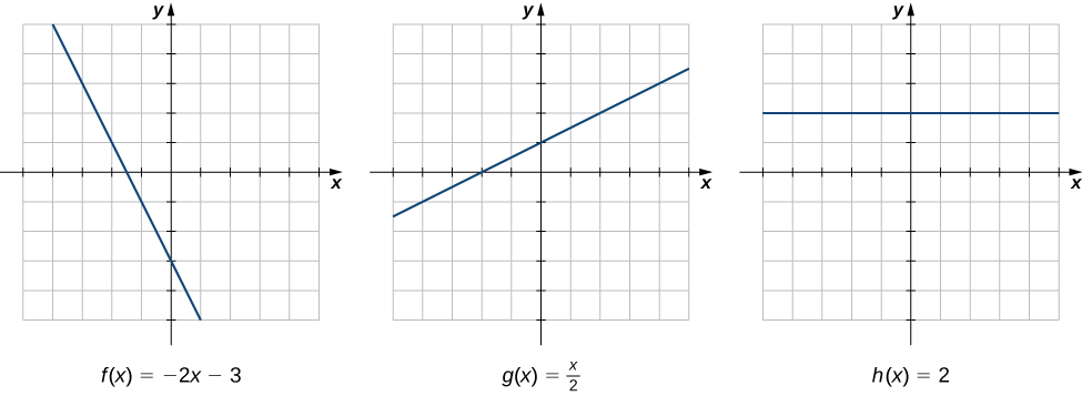
As we move from left to right along the graph of \(f(x)=−2x−3,\) we see that the graph decreases at a constant rate. For every 1 unit we move to the right along the \(x\)-axis, the \(y\)-coordinate decreases by 2 units. This rate of change is determined by the slope (−2) of the line. Similarly, the slope of 1/2 in the function \(g(x)\) tells us that for every change in \(x\) of 1 unit there is a corresponding change in \(y\) of 1/2 unit. The function \(h(x)=2\) has a slope of zero, indicating that the values of the function remain constant. We see that the slope of each linear function indicates the rate of change of the function.
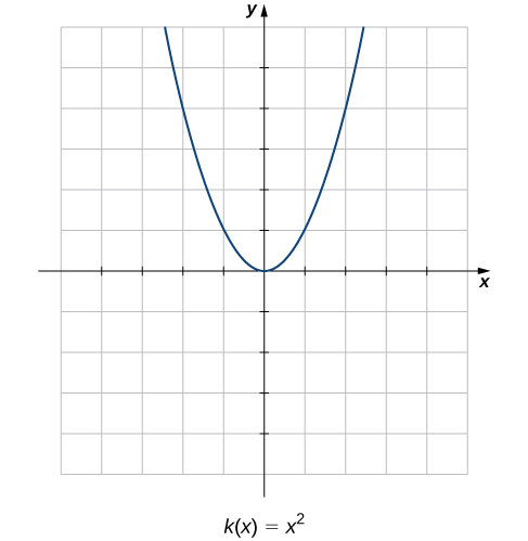
Compare the graphs of these three functions with the graph of \(k(x)=x^2\) (Figure 2.3). The graph of \(k(x)=x^2\) starts from the left by decreasing rapidly, then begins to decrease more slowly and level off, and then finally begins to increase—slowly at first, followed by an increasing rate of increase as it moves toward the right. Unlike a linear function, no single number represents the rate of change for this function. We quite naturally ask: How do we measure the rate of change of a nonlinear function?
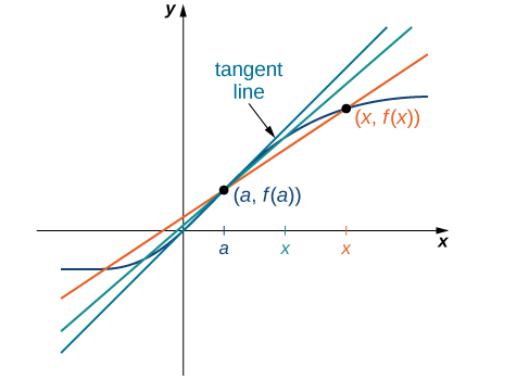
We can approximate the rate of change of a function \(f(x)\) at a point \((a,f(a))\) on its graph by taking another point \((x,f(x))\) on the graph of \(f(x),\) drawing a line through the two points, and calculating the slope of the resulting line. Such a line is called a secant line. Figure 2.4 shows a secant line to a function \(f(x)\) at a point \((a,f(a)).\)
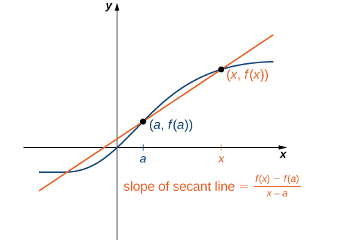
We formally define a secant line as follows:
Definition 2.5.
The secant to the function \(f(x)\) through the points \((a,f(a))\) and \((x,f(x))\) is the line passing through these points. Its slope is given by
The accuracy of approximating the rate of change of the function with a secant line depends on how close \(x\) is to \(a\text{.}\) As we see in Figure 2.6, if \(x\) is closer to \(a\text{,}\) the slope of the secant line is a better measure of the rate of change of \(f(x)\) at \(a\text{.}\)
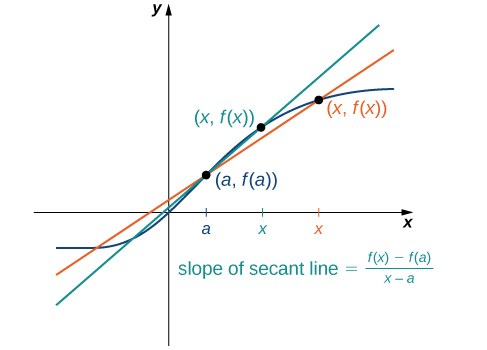
The secant lines themselves approach a line that is called the tangent to the function \(f(x)\) at \(a\) (Figure 2.8). The slope of the tangent line to the graph at \(a\) measures the rate of change of the function at \(a\text{.}\) This value also represents the derivative of the function \(f(x)\) at \(a\text{,}\) or the rate of change of the function at \(a\text{.}\) This derivative is denoted by \(f′(a).\) Differential calculus is the field of calculus concerned with the study of derivatives and their applications.
Note 2.7. Media.
For an interactive demonstration of the slope of a secant line that you can manipulate yourself, visit this applet (Note: this site requires a Java browser plugin): Math Insight 1 .
Example 2.9 illustrates how to find slopes of secant lines. These slopes estimate the slope of the tangent line or, equivalently, the rate of change of the function at the point at which the slopes are calculated.
Example 2.9. Finding Slopes of Secant Lines.
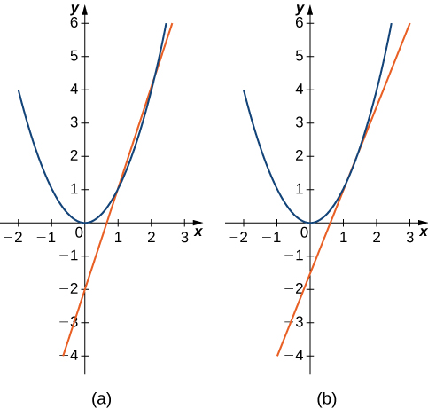
Estimate the slope of the tangent line (rate of change) to \(f(x)=x^2\) at \(x=1\) by finding slopes of secant lines through \((1,1)\) and each of the following points on the graph of \(f(x)=x^2.\)
\(\displaystyle (2,4)\)
\(\displaystyle (\frac{3}{2},\frac{9}{4})\)
Use the formula for the slope of a secant line from the definition.
\(\displaystyle m_{\sec}= \frac{4−1}{2−1}=3\)
\(\displaystyle m_{\sec}= \frac{\frac{9}{4}−1}{\frac{3}{2}−1}=\frac{5}{2}=2.5\)
The point in part b. is closer to the point \((1,1),\) so the slope of 2.5 is closer to the slope of the tangent line. A good estimate for the slope of the tangent would be in the range of 2 to 2.5 (Figure 2.10).
Checkpoint 2.11.
Estimate the slope of the tangent line (rate of change) to \(f(x)=x^2\) at \(x=1\) by finding slopes of secant lines through \((1,1)\) and the point \((\frac{5}{4},\frac{25}{16})\) on the graph of \(f(x)=x^2.\)
We continue our investigation by exploring a related question. Keeping in mind that velocity may be thought of as the rate of change of position, suppose that we have a function, \(s(t),\) that gives the position of an object along a coordinate axis at any given time \(t \text{.}\) Can we use these same ideas to create a reasonable definition of the instantaneous velocity at a given time \(t=a?\) We start by approximating the instantaneous velocity with an average velocity. First, recall that the speed of an object traveling at a constant rate is the ratio of the distance traveled to the length of time it has traveled. We define the average velocity of an object over a time period to be the change in its position divided by the length of the time period.
Definition 2.12.
Let \(s(t)\) be the position of an object moving along a coordinate axis at time \(t \text{.}\) The average velocity of the object over a time interval \([a,t]\) where \(a\lt t\) (or \([t,a]\) if \(t\lt a)\) is
As \(t \) is chosen closer to \(a\text{,}\) the average velocity becomes closer to the instantaneous velocity. Note that finding the average velocity of a position function over a time interval is essentially the same as finding the slope of a secant line to a function. Furthermore, to find the slope of a tangent line at a point \(a\text{,}\) we let the \(x\)-values approach \(a\) in the slope of the secant line. Similarly, to find the instantaneous velocity at time \(a\text{,}\) we let the \(t \)-values approach \(a\) in the average velocity. This process of letting \(x\) or \(t \) approach \(a\) in an expression is called taking a limit. Thus, we may define the instantaneous velocity as follows.
Definition 2.13.
For a position function \(s(t),\) the instantaneous velocity at a time \(t=a\) is the value that the average velocities approach on intervals of the form \([a,t]\) and \([t,a]\) as the values of \(t \) become closer to \(a\text{,}\) provided such a value exists.
Example 2.14 illustrates this concept of limits and average velocity.
Example 2.14. Finding Average Velocity.
A rock is dropped from a height of 64 ft. It is determined that its height (in feet) above ground \(t \) seconds later (for \(0≤t≤2)\) is given by \(s(t)=−16t^2+64.\) Find the average velocity of the rock over each of the given time intervals. Use this information to guess the instantaneous velocity of the rock at time \(t=0.5.\)
\(\displaystyle [0.49,0.5]\)
\(\displaystyle [0.5,0.51]\)
Substitute the data into the formula for the definition of average velocity.
\(\displaystyle v_{\text{ave}}= \frac{s(0.5)−s(0.49)}{0.5−0.49}=−15.84\)
\(\displaystyle v_{\text{ave}}= \frac{s(0.51)−s(0.5)}{0.51−0.5}=−16.16\)
The instantaneous velocity is somewhere between −15.84 and −16.16 ft/sec. A good guess might be −16 ft/sec.
Checkpoint 2.15.
An object moves along a coordinate axis so that its position at time \(t \) is given by \(s(t)=t^3.\) Estimate its instantaneous velocity at time \(t=2\) by computing its average velocity over the time interval \([2,2.001].\)
Subsection 2.1.2 The Area Problem and Integral Calculus
We now turn our attention to a classic question from calculus. Many quantities in physics—for example, quantities of work—may be interpreted as the area under a curve. This leads us to ask the question: How can we find the area between the graph of a function and the \(x\)-axis over an interval (Figure 2.16)?
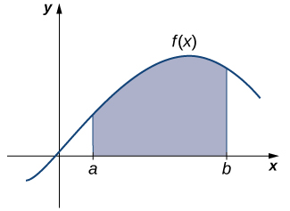
As in the answer to our previous questions on velocity, we first try to approximate the solution. We approximate the area by dividing up the interval \([a,b]\) into smaller intervals in the shape of rectangles. The approximation of the area comes from adding up the areas of these rectangles (Figure 2.17).
!["The graph is the same as the previous image, with one difference. Instead of the area completely shaded under the curved function, the interval [a, b] is divided into smaller intervals in the shape of rectangles. The rectangles have the same small width. The height of each rectangle is the height of the function at the midpoint of the base of that specific rectangle."](external/CNX_Calc_Figure_02_01_007.jpg)
As the widths of the rectangles become smaller (approach zero), the sums of the areas of the rectangles approach the area between the graph of \(f(x)\) and the \(x\)-axis over the interval \([a,b].\) Once again, we find ourselves taking a limit. Limits of this type serve as a basis for the definition of the definite integral. Integral calculus is the study of integrals and their applications.
Example 2.18. Estimation Using Rectangles.
Estimate the area between the \(x\)-axis and the graph of \(f(x)=x^2+1\) over the interval \([0,3]\) by using the three rectangles shown in Figure 2.19.
!["A graph of the parabola f(x) – x^2 + 1 drawn on graph paper with all units shown. The rectangles completely contained under the function and above the x-axis in the interval [0,3] are shaded. This strategy sets the heights of the rectangles as the smaller of the two corners that could intersect with the function. As such, the rectangles are shorter than the height of the function."](external/CNX_Calc_Figure_02_01_008.jpg)
The areas of the three rectangles are 1 unit\(^2\text{,}\) 2 unit\(^2\text{,}\) and 5 unit\(^2\text{.}\) Using these rectangles, our area estimate is 8 unit\(^2\text{.}\)
Checkpoint 2.20.
Estimate the area between the \(x\)-axis and the graph of \(f(x)=x^2+1\) over the interval \([0,3]\) by using the three rectangles shown here:
!["A graph of the same parabola f(x) = x^2 + 1, but with a different shading strategy over the interval [0,3]. This time, the shaded rectangles are given the height of the taller corner that could intersect with the function. As such, the rectangles go higher than the height of the function](external/CNX_Calc_Figure_02_01_009.jpg)
Subsection 2.1.3 Other Aspects of Calculus
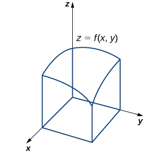
So far, we have studied functions of one variable only. Such functions can be represented visually using graphs in two dimensions; however, there is no good reason to restrict our investigation to two dimensions. Suppose, for example, that instead of determining the velocity of an object moving along a coordinate axis, we want to determine the velocity of a rock fired from a catapult at a given time, or of an airplane moving in three dimensions. We might want to graph real-value functions of two variables or determine volumes of solids of the type shown in Figure 2.21. These are only a few of the types of questions that can be asked and answered using multivariable calculus. Informally, multivariable calculus can be characterized as the study of the calculus of functions of two or more variables. However, before exploring these and other ideas, we must first lay a foundation for the study of calculus in one variable by exploring the concept of a limit.
Subsection 2.1.4 Key Concepts
Differential calculus arose from trying to solve the problem of determining the slope of a line tangent to a curve at a point. The slope of the tangent line indicates the rate of change of the function, also called the derivative. Calculating a derivative requires finding a limit.
Integral calculus arose from trying to solve the problem of finding the area of a region between the graph of a function and the \(x\)-axis. We can approximate the area by dividing it into thin rectangles and summing the areas of these rectangles. This summation leads to the value of a function called the integral. The integral is also calculated by finding a limit and, in fact, is related to the derivative of a function.
Multivariable calculus enables us to solve problems in three-dimensional space, including determining motion in space and finding volumes of solids.
Subsection 2.1.5 Key Equations
Slope of a Secant Line \(m_{\sec}= \frac{f(x)−f(a)}{x−a}\)
Average Velocity over Interval \([a,t]\) \(v_{\text{ave}}=\frac{s(t)−s(a)}{t−a}\)
This book is a custom edition based on OpenStax Calculus Volume 1. You can download the original for free at https://openstax.org/details/books/calculus-volume-1.
openstax.org/l/20_mathinsight